EXPERIMENTS IN SUPERVISED LEARNING PART 4

Speeding up the Training Loop

When developing and evaluating different machine learning models, rapid iteration is key—especially as experiments shift from feature engineering to focused model evaluation. At this stage, we want to make it as fast as possible to rerun training and testing cycles, particularly since feature extraction can become a bottleneck if performed repeatedly on the same data. To save time (often 30 seconds or more per run), we can serialize and cache extracted features so that model evaluations proceed much faster. We will use the pickle library to serialize our data (which is a binary serialization format and not related to PickleBall in any way). As always, you can follow along by doing:

git checkout post-4-part-1

A simple check is added at the top of load_labeled_blocks to see if a pickled feature file already exists. If it does, the features are loaded directly from disk; otherwise, they are generated and then saved for next time.

cache_file = os.path.join(CACHE_DIR, f"labeled_blocks_limit_{limit}.pkl")

if os.path.exists(cache_file):
    with open(cache_file, "rb") as f:
        return pickle.load(f)

If no pickled file is found, the blocks are labeled as usual, and then the labeled features and targets are saved to disk for future runs using pickle.

with open(cache_file, "wb") as f:
    pickle.dump((X, y), f)

Because the end goal is to run this as a web service, it’s important to monitor and manage memory usage during prediction. To help with this, memory profiling and timing have been added to predict.py to track resource consumption each time the model is run.

When the LogisticRegression classifier is trained and evaluated on the entire dataset, the following performance metrics are obtained:

Evaluating...
              precision    recall  f1-score   support

   direction       0.63      0.77      0.69     10196
  ingredient       0.72      0.88      0.79     21496
        none       0.98      0.97      0.98    422226
       title       0.57      0.62      0.60      4308

    accuracy                           0.96    458226
   macro avg       0.73      0.81      0.76    458226
weighted avg       0.96      0.96      0.96    458226

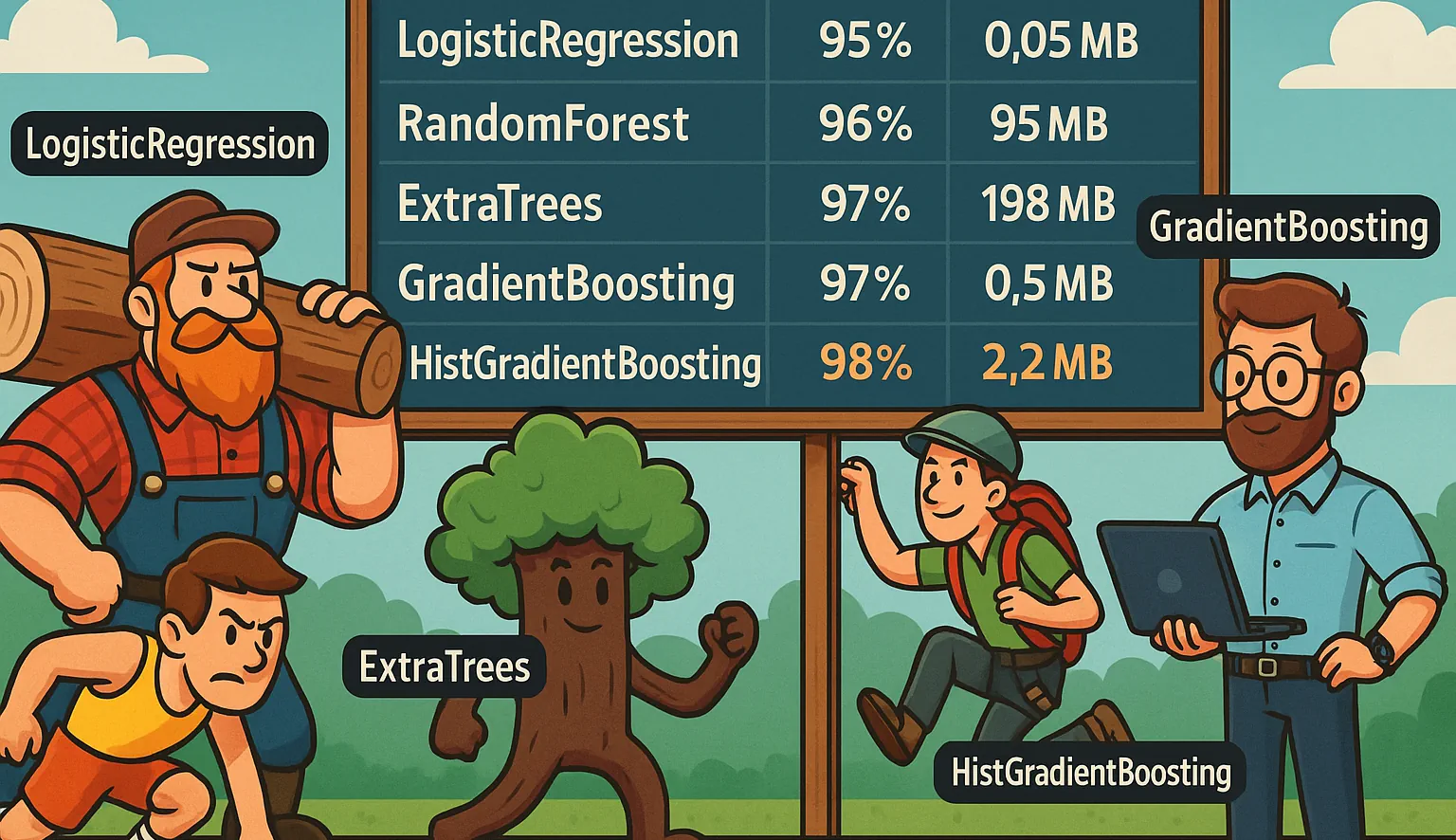
Model saved to model.joblib with a size of 0.053 MB

When the prediction script is run on a sample HTML file, the extracted results are generally quite accurate, though some imperfections still remain.

python.exe predict.py --memory ../data/html/crab-cakes.html 
{
  "title": "Maryland Crab Cakes",
  "ingredients": [
    "For the Crab Cakes",
    "2 large eggs",
    "2½ tablespoons mayonnaise, best quality such as Hellmann's or Duke's",
    "1½ teaspoons Dijon mustard",
    "1 teaspoon Worcestershire sauce",
    "1 teaspoon Old Bay seasoning",
    "¼ teaspoon salt",
    "¼ cup finely diced celery, from one stalk",
    "2 tablespoons finely chopped fresh parsley",
    "1 pound lump crab meat (see note below)",
    "½ cup panko",
    "Vegetable or canola oil, for cooking",
    "For the Quick Tartar Sauce",
    "1 cup mayonnaise, best quality such as Hellmann's or Duke's",
    "1½ tablespoons sweet pickle relish",
    "1 teaspoon Dijon mustard",
    "1 tablespoon minced red onion",
    "1-2 tablespoons lemon juice, to taste",
    "Salt and freshly ground black pepper, to taste",
    "For the Crab Cakes",
    "For the Quick Tartar Sauce",
    "Sugar: 1 g"
  ],
  "directions": [
    "To begin, combine the eggs, mayonnaise, Dijon mustard, Worcestershire, Old Bay, salt, celery, and parsley in a bowl.",
    "Mix well to combine.",
    "Add the crab meat, making sure to check for any hard and sharp cartilage as you go, along with the panko.",
    "Shape into 6 large cakes about ½ cup each, and place on a foil-lined baking sheet for easy cleanup. Then cover and refrigerate for at least 1 hour. This step is really important to help the crab cakes set, otherwise they may fall apart a bit when you cook them.",
    "Preheat a large nonstick pan to medium heat and coat with oil. When the oil is hot, place crab cakes in the pan and cook until golden brown, about 3 to 5 minutes.",
    "Flip and cook 3 to 5 minutes more, or until golden. Be careful as the oil may splatter.",
    "Next, make the tartar sauce by combining the mayonnaise, Dijon mustard, sweet pickle relish, red onion, lemon, salt, and pepper in a small bowl.",
    "Whisk well, then cover and chill until ready to serve.",
    ", plus at least 1 hour to let the crab cakes set",
    "Combine the eggs, mayonnaise, Dijon mustard, Worcestershire, Old Bay, salt, celery, and parsley in a large bowl and mix well. Add the crab meat (be sure to check the meat for any hard and sharp cartilage) and panko; using a rubber spatula, gently fold the mixture together until just combined, being careful not to shred the crab meat. Shape into 6 cakes (each about ½ cup) and place on the prepared baking sheet. Cover and refrigerate for at least 1 hour. This helps them set.",
    "Preheat a large nonstick pan over medium heat and coat with oil. When the oil is hot, place the crab cakes in the pan and cook until golden brown, 3 to 5 minutes per side. Be careful as oil may splatter. Serve the crab cakes warm with the tartar sauce.",
    "In a small bowl, whisk together the mayonnaise, relish, mustard, onion, and lemon juice. Season with salt and pepper, to taste. Cover and chill until ready to serve.",
    "Make-Ahead Instructions: The crab cakes can be formed, covered, and refrigerated a day ahead of time before cooking. The tartar sauce can be made and refrigerated up to 2 days in advance.",
    "Note: If you can only find jumbo lump crab meat, you may need to break the pieces up a bit. If the clumps are too large, the crab cakes won't hold together well.",
    "Note: The nutritional information does not include the tartar sauce."
  ]
}
Peak memory from tracemalloc: 7.85 MB
Total memory usage from psutil: 158.40 MB
Memory increase: 15.11 MB
️Total time: 0.35s

Up to this point, the machine learning pipeline has essentially been treated as a black box—relying on the default choices for both the Transformer and Classifier commonly used in supervised learning tasks with labeled data. However, to better understand and improve performance, it's worth taking a closer look at how the Transformer and Classifier actually work.

Our Transformer

Let’s take a closer look at how the transformer in our pipeline is constructed and why it’s set up this way.

transformer = FeatureUnion([
    ("structured", make_pipeline(ItemSelector('structured'), dict_vect)),
    ("text", make_pipeline(ItemSelector('text'), TfidfVectorizer(max_features=500, ngram_range=(1, 2))))
])

The FeatureUnion in this pipeline allows both structured data (such as manually engineered features from previous steps like labeling and balancing) and unstructured text to be processed in parallel. Structured features are handled by a dictionary vectorizer, while the raw text is transformed using a TfidfVectorizer. The ItemSelector class is used to extract the correct part of each data sample for the appropriate transformation, ensuring that both types of features are efficiently combined for model training.

class ItemSelector(BaseEstimator, TransformerMixin):
    def __init__(self, key: str):
        self.key = key

    def fit(self, X: List[Any], y: Any = None) -> 'ItemSelector':
        return self

    def transform(self, X: List[Tuple[Dict[str, Any], str]]) -> List[Union[Dict[str, Any], str]]:    
        if self.key == 'structured':
            return [x[0] for x in X]  # structured features (dict)
        elif self.key == 'text':
            return [x[1] for x in X]  # text field
        else:
            raise ValueError(f"Unknown key: {self.key}")

TF-IDF, or Term Frequency-Inverse Document Frequency, is a classic technique for transforming raw text into a structured format that machine learning algorithms can understand. The process creates a matrix where each feature corresponds to a word (or phrase) and reflects its importance in a document compared to the rest of the corpus. This is achieved by multiplying two measures: term frequency (how often an n-gram appears in a given document) and inverse document frequency (how rare that n-gram is across all documents). As a result, frequently occurring but uninformative words (such as "the" and "and") receive lower scores, while rare and distinctive words are emphasized. This transformation forms the core of the text-based feature engineering in our NLP pipeline.

The max_features parameter controls how many unique n-grams are tracked by the vectorizer. In our setup, only the top 500 most frequent and informative n-grams are kept. This helps manage memory usage and model complexity, while also reducing the risk of overfitting to rare patterns or noise.

The ngram_range parameter specifies the size of word groups (n-grams) considered by the vectorizer. In this configuration, both unigrams (single words) and bigrams (pairs of consecutive words) are extracted as features, enabling the model to capture not only individual word importance but also common word combinations that may signal important structure in recipes.

In short, our transformer combines both structured metadata and text features from each recipe, turning them into a single, unified feature set. This setup allows the machine learning model to learn from both the explicit structure of the recipe and the subtle patterns in the ingredient and direction text, maximizing its ability to accurately classify recipe elements.

Our Classifier

model = make_pipeline(
    build_transformer(),
    StandardScaler(with_mean=False),
    LogisticRegression(solver='lbfgs', max_iter=1000)
)

The core of our model is a LogisticRegression classifier, configured with the lbfgs solver. But what is a LogisticalRegression classifier? Despite what the name suggests, LogisticRegression is actually designed for classification tasks. Its goal is to estimate the probability (between 0 and 1) that a given input should be assigned to a particular class, using a sigmoid function to map predictions to probabilities.

$\sigma(x) = \frac{1}{1 + e^{-x}}$

for the formulae:

$P(\text{c}=1 \mid x) = \sigma(w_1 x_1 + w_2 x_2 + \ldots + w_n x_n + b)$

In this equation, the x variables represent the TF-IDF features extracted from each input. Each feature is multiplied by a learned weight (produced by the solver), and a bias term is added to the sum. The bias serves as a baseline probability—essentially, it represents the model's prediction when all input features are zero.

But what about the solver? We know it produces the weights and bias—but how does it actually accomplish this? The answer: it searches for the set of parameters that minimizes the loss function (a measure of how incorrect the model's predictions are). This approach is fundamental to all solvers used in logistic regression.

How Does It Work?

Start by initializing all the parameters (weights and bias), to either zeros, or small random numbers.
Compute the loss (e.g., “How far off are my predictions?”).
Compute the gradient (i.e., “If I change each parameter a little, how does the loss change?”).
Figure out a direction to step in for each parameter to make the loss go down, using information about the curvature of the loss function (second derivatives, also called the Hessian.
Update all parameters in a way that’s smarter and usually faster than just following the steepest descent (simple gradient descent).
Repeat steps 2-5 until the changes are tiny (the model is “converged”), or you reach a max number of steps.

How exactly does lbfgs do this? That is math above my understanding of calculus and linear algebra, but as long as we understanding what it is doing we don't really need to understand exactly how it does it, but if you want a much deeper explanation of Solvers look at Scikit-learn solvers explained. I tried swapping out the various solvers (liblinear, newtoncg, newton-cholesky) and they produced the same results but were either or slower or used a lot more memory (sag and saga never worked on the small dataset, as expected, but I wasn't patient enough after waiting a couple of hours for it work on the full dataset).

So how does lbfgs actually work under the hood? The answer involves some advanced calculus and linear algebra—territory that isn’t required for practical use, as long as you have a general understanding of what it accomplishes. If you’re curious about the mathematical details, I recommend this breakdown: Scikit-learn solvers explained.

For my experiments, I tried swapping out a variety of solvers (liblinear, newtoncg, and newton-cholesky). All produced similar results, but some were noticeably slower or used much more memory. The 'sag' and 'saga' solvers never worked well on the small dataset (as expected), and I wasn't patient enough to wait several hours for them to finish processing on the full dataset.

RandomForestClassifier

Let's explore changing our classifier. The first alternative we'll try is the RandomForestClassifier, a powerful and widely-used ensemble learning method.

git checkout post-4-part-2

Notice that the only change we made was swapping out the classifier. We also no longer need the StandardScaler, since RandomForestClassifier can handle sparse data directly:

print("Training model...")
model = make_pipeline(
    build_transformer(),
    RandomForestClassifier(random_state=42)
)

After training our model with RandomForestClassifier, the results are immediately impressive.

Evaluating...
              precision    recall  f1-score   support

   direction       0.62      0.85      0.72       885
  ingredient       0.74      0.94      0.83      1726
        none       0.99      0.97      0.98     39269
       title       0.68      0.70      0.69       396

    accuracy                           0.96     42276
   macro avg       0.76      0.86      0.80     42276
weighted avg       0.97      0.96      0.97     42276

Model saved to model.joblib with a size of 94.519 MB

However, there's a major trade-off: our model size jumps dramatically—from just 50 KB to nearly 100 MB. And if we train on the entire dataset, the model can swell to over 2 GB.

So, what exactly is a RandomForestClassifier? Unlike LogisticRegression, which makes predictions based on a single mathematical function, RandomForestClassifier is an ensemble method that builds many independent decision trees and aggregates their predictions. Each tree in the forest casts a “vote” for a class, and the class with the most votes is chosen as the final prediction.

During training, RandomForestClassifier constructs hundreds or even thousands of decision trees. Each tree is trained on a random subset of your data (a process known as bagging), and at each decision split, it only considers a random subset of features. This randomness helps ensure that the trees are diverse and not overly correlated with one another.

During prediction, the model runs each sample through every tree in the forest. Each tree makes its own classification, and the class that receives the most "votes" across all trees becomes the final prediction. If desired, RandomForestClassifier can also output the probability distribution over all classes (rather than just a single predicted label), though this pipeline, only the top class is returned.

But this improved accuracy comes at a significant cost: increased disk space and memory usage during prediction. Fortunately, we can manage model size by carefully tuning a few key parameters.

The first parameter to consider is the number of trees in the forest (n_estimators). When I set this to 200, the model size doubled. Using 100 trees kept the model about the same size. (The default number of trees can change depending on the dataset, but for our limited dataset, it was about 100.) Reducing the count to 75 trees made the model smaller, with only a slight dip in accuracy—mainly in the 'direction' category:

             precision    recall  f1-score   support

   direction       0.61      0.84      0.71       885
  ingredient       0.74      0.95      0.83      1726
        none       0.99      0.97      0.98     39269
       title       0.68      0.70      0.69       396

    accuracy                           0.96     42276
   macro avg       0.76      0.87      0.80     42276
weighted avg       0.97      0.96      0.97     42276

Model saved to model.joblib with a size of 70.981 MB

Another important parameter is max_depth, which controls how deep each tree can grow. Reducing max_depth produces much shallower trees and leads to a significant decrease in model size, with only minimal impact on accuracy. For instance, setting max_depth to 20 (while reverting n_estimators) results in a model just 19 MB in size—still with strong performance.

              precision    recall  f1-score   support

   direction       0.62      0.75      0.68       885
  ingredient       0.74      0.87      0.80      1726
        none       0.98      0.98      0.98     39269
       title       0.79      0.35      0.49       396

    accuracy                           0.96     42276
   macro avg       0.78      0.74      0.74     42276
weighted avg       0.96      0.96      0.96     42276

Model saved to model.joblib with a size of 19.052 MB

Adjusting min_samples_leaf to 2 (which sets the minimum number of samples required in each leaf node) allows us to reduce model size even further while preserving most of the accuracy.

              precision    recall  f1-score   support

   direction       0.61      0.79      0.69       885
  ingredient       0.74      0.91      0.82      1726
        none       0.99      0.97      0.98     39269
       title       0.75      0.59      0.66       396

    accuracy                           0.96     42276
   macro avg       0.77      0.82      0.79     42276
weighted avg       0.97      0.96      0.96     42276

Model saved to model.joblib with a size of 33.110 MB

By combining these parameter tweaks, we can reduce the model size to a manageable 13.3 MB with only a minimal drop in accuracy:

    model = make_pipeline(
        build_transformer(),
        RandomForestClassifier(random_state=42, min_samples_leaf=2, n_estimators=80, max_depth=25),
    )

which produces:

              precision    recall  f1-score   support

   direction       0.63      0.77      0.69       885
  ingredient       0.73      0.89      0.80      1726
        none       0.98      0.97      0.98     39269
       title       0.78      0.46      0.58       396

    accuracy                           0.96     42276
   macro avg       0.78      0.77      0.76     42276
weighted avg       0.96      0.96      0.96     42276

Model saved to model.joblib with a size of 13.337 MB

This is an effective balance between model accuracy and size—striking a practical trade-off for real-world use. In summary: RandomForestClassifier can greatly improve results, but requires careful parameter tuning to avoid ballooning model sizes.

ExtraTreesClassifier

Another option is the ExtraTreesClassifier. While we won’t focus much on it here—since it tends to produce extremely large models—it’s worth a brief mention.

The ExtraTreesClassifier (short for Extremely Randomized Trees) is another ensemble method, closely related to RandomForestClassifier. Both build a forest of decision trees using random subsets of data (bootstrapping), but ExtraTrees introduces an extra layer of randomness: at each split in a tree, it chooses the split threshold completely at random from possible values, rather than searching for the most optimal split among selected features. This approach can speed up training, but also tends to increase the overall model size.

model = make_pipeline(
    build_transformer(),
    ExtraTreesClassifier(random_state=42),
)

However, because the initial model size is so large, we won’t spend time trying to tune it for practical use. It’s included here mainly to illustrate another example of a supervised learning classifier.

              precision    recall  f1-score   support

   direction       0.59      0.85      0.70       885
  ingredient       0.72      0.94      0.82      1726
        none       0.99      0.97      0.98     39269
       title       0.64      0.72      0.68       396

    accuracy                           0.96     42276
   macro avg       0.74      0.87      0.79     42276
weighted avg       0.97      0.96      0.96     42276

Model saved to model.joblib with a size of 198.425 MB

While the ExtraTreesClassifier can offer strong performance, but its significant model size makes it impractical for many real-world applications. While its additional randomness can speed up training, the storage and deployment costs generally outweigh the benefits unless you have a specific use case that justifies the extra size.

GradientBoostingClassifier

The GradientBoostingClassifier is a different kind of decision tree ensemble. Rather than building many trees in parallel (like RandomForestClassifier), it builds them sequentially, where each new tree tries to correct the errors of the previous trees. This process is called boosting: every new tree “boosts” the model’s performance by focusing on the mistakes made so far.

Let’s take a closer look at what happens when we use GradientBoostingClassifier in practice.

git checkout post-4-part-3

Thanks to this sequential, error-correcting approach, GradientBoostingClassifier delivers strong performance with a much smaller model size than RandomForestClassifier—often matching or even surpassing its results in just half a megabyte. The trade-off is that training typically takes longer.

              precision    recall  f1-score   support

   direction       0.61      0.76      0.68       885
  ingredient       0.72      0.90      0.80      1726
        none       0.99      0.97      0.98     39269
       title       0.66      0.58      0.62       396

    accuracy                           0.96     42276
   macro avg       0.74      0.80      0.77     42276
weighted avg       0.96      0.96      0.96     42276

Model saved to model.joblib with a size of 0.522 MB

We can further tune the model by increasing the max_depth parameter—allowing each tree to grow deeper and better capture complex patterns. For example, raising max_depth from the default value of 5 up to 7,

model = make_pipeline(
    build_transformer(),
    GradientBoostingClassifier(random_state=42, max_depth=7),
)

this results in even better accuracy, though the model size does increase by a few megabytes:

              precision    recall  f1-score   support

   direction       0.62      0.82      0.70       885
  ingredient       0.74      0.92      0.82      1726
        none       0.99      0.97      0.98     39269
       title       0.60      0.67      0.64       396

    accuracy                           0.96     42276
   macro avg       0.74      0.85      0.78     42276
weighted avg       0.97      0.96      0.96     42276

Model saved to model.joblib with a size of 3.403 MB

Overall, GradientBoostingClassifier offers an appealing balance of high accuracy and compact model size, making it a strong choice for many real-world scenarios where storage and deployment constraints matter. Its sequential training allows it to adapt and improve with each tree, but this power comes at the cost of slower training times compared to parallel methods like RandomForestClassifier. If your primary concern is model size without sacrificing much performance, GradientBoostingClassifier is well worth considering.

HistGradientBoostingClassifier

The HistGradientBoostingClassifier is another type of gradient boosting classifier, similar to GradientBoostingClassifier, but it introduces a powerful optimization: feature binning. Feature binning groups continuous feature values into discrete bins, which makes training much faster and uses less memory, especially on large datasets.

To use this classifier, we need to make a couple of small adjustments to our code. First, we add the Densify class to feature_extraction.py (and import it in both train.py and predict.py).

git checkout post-4-part-4

Here is the densify class we required:

class Densify(TransformerMixin):
    def fit(self, X, y=None):
        return self
    def transform(self, X, y=None):
        return X.toarray()

Then add it to the imports:

from feature_extraction import extract_features, build_transformer, preprocess_data, get_section_header, Densify

Next, incorporate the HistGradientBoostingClassifier into our pipeline:

model = make_pipeline(
    build_transformer(),
    Densify(),
    HistGradientBoostingClassifier(
        random_state=42
    )
)

Finally, be sure to add the import to your predict.py script (this is necessary if you want to actually use the model for prediction—since the class is instantiated when the model loads).

When we train and evaluate this model, it delivers our strongest results so far—all in a highly compact 2.4 MB package.

              precision    recall  f1-score   support

   direction       0.62      0.84      0.71       885
  ingredient       0.73      0.93      0.82      1726
        none       0.99      0.97      0.98     39269
       title       0.65      0.74      0.69       396

    accuracy                           0.96     42276
   macro avg       0.75      0.87      0.80     42276
weighted avg       0.97      0.96      0.97     42276

Model saved to model.joblib with a size of 2.253 MB

In summary, HistGradientBoostingClassifier stands out for its efficiency and accuracy. By leveraging feature binning, it achieves excellent results while keeping the model size very compact—making it a great choice for large datasets or production environments where memory usage matters.

There are more classifiers to try:

LinearSVC — A linear support vector machine classifier, which works well for high-dimensional sparse data and is similar in spirit to LogisticRegression, but uses a different optimization approach.
DecisionTreeClassifier — A basic tree-based classifier that is extremely fast and interpretable, making it well-suited for small or simple datasets. However, it can struggle with complex data and is prone to overfitting unless regularization techniques are used.
XGBoost — A widely used, highly optimized gradient boosting framework that is often considered state-of-the-art in machine learning competitions. While it’s not included in scikit-learn by default and requires extra setup, XGBoost is extremely flexible and powerful. However, in this particular use case, it actually performed slightly worse than both GradientBoostingClassifier and HistGradientBoostingClassifier.
MLPClassifier — A feedforward neural network classifier (multi-layer perceptron) that can model complex, nonlinear relationships. MLPClassifier offers a lot of flexibility and power, but it comes with many configuration options and typically requires extensive tuning to achieve optimal performance. It can be a fascinating option to experiment with if you're interested in neural networks.

Things to try:

Try adjusting the parameters of HistGradientBoostingClassifier (such as max_iter, learning_rate, or max_leaf_nodes) to see if you can push the accuracy even higher, while still keeping the model size manageable.
Challenge yourself to get XGBoost or the MLPClassifier running in your pipeline and compare their results to the classifiers above.
Experiment with the TfidfVectorizer parameters—such as max_features, ngram_range, or even min_df—to see how they impact both accuracy and model size. Tweaking these options can help you find the best trade-off for your particular dataset and task.

Expanding to the Full Training Set

When we train the HistGradientBoostingClassifier on the full dataset, the results are quite similar to those from the limited training set, with only slight improvements in performance. Interestingly, instead of the model size increasing, it actually decreased.

              precision    recall  f1-score   support

   direction       0.64      0.84      0.73     10196
  ingredient       0.74      0.92      0.82     21496
        none       0.99      0.97      0.98    422226
       title       0.62      0.73      0.67      4308

    accuracy                           0.96    458226
   macro avg       0.75      0.86      0.80    458226
weighted avg       0.97      0.96      0.96    458226

Model saved to model.joblib with a size of 1.799 MB

This happens because HistGradientBoostingClassifier uses a fixed number of bins to discretize continuous feature values, and the size of the model is determined mainly by hyperparameters such as the number of boosting stages and the tree structure (not the number of samples). With more data, the trees may even become more efficient—sometimes pruning unnecessary splits—leading to a smaller model file overall. Unlike some other algorithms that grow with data size, histogram-based methods remain compact and stable as your dataset scales.

After trying out a variety of classifiers, some key differences stand out. If you need something that trains lightning fast, produces tiny models, and gives you interpretable results, LogisticRegression is a fantastic place to start. It's hard to beat for simple, linearly separable problems or as a quick baseline.

But if your data is more complicated and you want a model that can capture those nonlinear patterns, RandomForestClassifier is like the Swiss Army knife of classifiers. It delivers strong, reliable performance on a wide range of problems—just be prepared for much bigger model files. And if you want even more randomness (sometimes at the cost of accuracy and definitely at the cost of file size), ExtraTreesClassifier is worth a look, but it’s generally best for experimenting or ensemble models where space isn’t a concern.

GradientBoostingClassifier takes a different approach: it builds trees sequentially, with each new tree focusing on fixing the mistakes of the last. The payoff is that you often get just as much accuracy as RandomForest, but packed into a much smaller model—especially if you’re willing to spend some extra time tuning.

And finally, the star of the show for big datasets and production use: HistGradientBoostingClassifier. Thanks to its feature binning trick, it keeps models compact and training fast, no matter how much data you throw at it. If storage and memory matter to you (and let’s be honest, they usually do in production), this is the one to beat.

In short, start with LogisticRegression if you want speed and simplicity, try RandomForest when you need power and don’t care about size, and reach for GradientBoosting or HistGradientBoosting when you want a compact, high-performing model that scales well.

Final Code Improvements - Post Processing

Even after all our modeling work, a few annoying artifacts slip through. For example, you’ll sometimes find things like "Sugar: 1 g" or "Carbohydrates: 9 g" showing up as ingredients—this happens almost 30,000 times in our dataset! Similarly, lines like "For the Crab Cakes" or "For the Tartar Sauce" (which appear over 4,000 times) are section headers, not true ingredients. Rather than retrain the entire model to catch these rare, formulaic patterns, the most practical fix is a little post-processing cleanup. This way, we can quickly filter them out after prediction, keeping our ingredient lists clean without complicating the training pipeline.

git checkout post-4-part-5

To address this, we simply update our predict.py file with the following code:

SECTION_HEADING_PATTERN = re.compile(
    r"^for the ",
    re.IGNORECASE,
)

NUTRITION_PATTERN = re.compile(
    r"^(calories|fat|saturated fat|carbohydrates|sugar|fiber|protein|sodium|cholesterol)[:\\-]\s*\d+",
    re.IGNORECASE,
)

def is_fake_ingredient(text):
    text = text.strip()
    if SECTION_HEADING_PATTERN.match(text):
        return True
    if NUTRITION_PATTERN.match(text):
        return True
    return False

Next, we tweak our extract_structured_data function to check whether each candidate ingredient matches our 'fake ingredient' patterns before adding it to the list. This helps us skip over section headers and nutritional info lines, ensuring our ingredient lists only include true ingredients.

    structured = {"title": None, "ingredients": [], "directions": []}
    for el, label in zip(elements, predictions):
        text = el["text"]
        if label == "title" and structured["title"] is None:
            structured["title"] = text
        elif label == "ingredient":
            if is_fake_ingredient(text):
                continue
            structured["ingredients"].append(text)

Why use post-processing to filter out “For the” section headers and nutritional info as ingredients?

These lines are really just part of the recipe’s formatting or layout (“UI/UX artifacts”), not true data about the recipe itself. Lines like “For the Topping,” “For the Sauce,” or “Calories: 200” are actually section markers or nutrition notes written for the reader. They’re often presented in a way—such as in a list, styled like an ingredient—that can fool both humans and ML models into thinking they’re real ingredients.

Luckily, these cases are both rare and highly predictable—they follow very consistent patterns like “For the ...” or “Calories: ...”. That means a simple regex or string-match filter will catch almost all of them, and you only need a few lines of code to keep your results clean.

Trying to fix this by relabeling your training data is a huge headache—you'd need to manually relabel thousands of recipe files, which is tedious and likely to introduce mistakes. Worse, you might end up with inconsistent labels, where some recipes mark these lines as 'ingredient' and others don't. Even after all that work, the model could still get confused and misclassify these lines, because their features can look almost identical to real ingredients—especially in a generic machine learning pipeline.

The goal is for your model to generalize, not memorize specific quirks. If you hard-code a rule in your training data like “never predict ingredient if the text is ‘For the X’,” you risk your model missing legitimate ingredients in new or different formats. It’s better to keep your model focused on learning the general concept of what makes an ingredient, rather than overfitting to a handful of edge cases.

Post-processing is fast, transparent, and easy to update. If you need to add or remove patterns, it's as simple as tweaking a regex or list in your code—no retraining required. And if you spot a new false positive, you can filter it out instantly, with zero impact on your machine learning logic.

Things to try

Try running python src/predict.py --memory ../data/html_pages/recipe_00004.html on recipe_00004.html and several other recipes from the data_html folder—or any other recipes you’re curious about. As you review the outputs, see if you spot any other abnormal artifacts (like repeated directions or ingredient doubling) that could be cleaned up with more post-processing rules.
Now, try running python src/predict.py --memory ../data/html/recipe_00038.html. You'll notice that the extracted title is "Gluten-Free Chocolate Cake Cookies," but it should actually be "Gluten-Free Angel Food Cake Recipe." When you see issues like this, consider: is it something best solved by improving your model, or can you handle it more effectively with post-processing give that we literally have the correct recipe name in the html's <title/> tag.

Creating a Prediction Service

Now that our model is performing well, let’s take it a step further and make it available as a web service so others (or our own applications) can use it easily.

git checkout post-4-part-6

To make this work efficiently, we need to refactor how we use predict.py and the extract_structured_data function. Rather than reloading the model for every request (which would quickly bog down our web service), we'll load the model once at startup and reuse it for each incoming request. Also, instead of reading HTML files from disk within our prediction code, we'll pass in the HTML text directly—giving our service the flexibility to accept any HTML input it receives.

Here’s what the core service logic looks like after these changes:

recipeModel = load(MODEL_PATH)
html = Path(args.html_path).read_text(encoding="utf-8")

result = extract_structured_data(html, recipeModel)
print(json.dumps(result, indent=2, ensure_ascii=False))

Here’s the improved and much simpler extract_structured_data function:

elements = parse_html(html)
all_features = []
current_section_heading = None  # Track current section heading
for idx, el in enumerate(elements):

    current_section_heading = get_section_header(current_section_heading, el)

    features = extract_features(el, idx, elements, current_section_heading)
    all_features.append(features)

data = preprocess_data(all_features)

predictions = model.predict(data)

Next, let’s update our requirements. We’ll use FastAPI because it’s fast, modern, and perfect for building new Python APIs. Uvicorn will be our high-performance ASGI server, and python-multipart makes it easy to handle file uploads. Just add these lines to your requirements.txt:

fastapi~=0.115.14
uvicorn~=0.34.3
python-multipart~=0.0.20

With those dependencies in place, building the web service with FastAPI is refreshingly straightforward:

from fastapi import FastAPI, UploadFile, File
from fastapi.responses import JSONResponse
from joblib import load

from predict import extract_structured_data
from config import MODEL_PATH

# PRELOAD model at startup
recipeModel = load(MODEL_PATH)

app = FastAPI()

@app.post("/predict")
async def predict(html: UploadFile = File(...)):
    html_text = (await html.read()).decode("utf-8")
    result = extract_structured_data(html_text, recipeModel)
    return JSONResponse(result)

Start the service locally with this command:

$ uvicorn predict_service:app --host 127.0.0.1 --port 8000

One of the best parts about FastAPI is that it automatically gives you a user-friendly, interactive API explorer at http://127.0.0.1:8000/docs, making it easy to experiment with your endpoint right in the browser but it also lets you know that it is up and running. You can also test it out from the command line (in the root of our project):

$ curl -X POST -F "html=@data/html/crab-cakes$.html" http://127.0.0.1:8000/predict

You should see output like this:

$ curl -X POST -F "html=@data/html/crab-cakes.html" http://127.0.0.1:8000/predict 
{"title":"Maryland Crab Cakes","ingredients":["2 large eggs","2½ tablespoons mayonnaise, best quality such as Hellmann's or Duke's","1½ teaspoons Dijon mustard","1 teaspoon Worcestershire sauce","1 teaspoon Old Bay seasoning","¼ teaspoon salt","¼ cup finely diced celery, from one stalk","2 tablespoons finely chopped fresh parsley","1 pound lump crab meat (see note below)","½ cup panko","Vegetable or canola oil, for cooking","1 cup mayonnaise, best quality such as Hellmann's or Duke's","1½ tablespoons sweet pickle relish","1 teaspoon Dijon mustard","1 tablespoon minced red onion","1-2 tablespoons lemon juice, to taste","Salt and freshly ground black pepper, to taste"],"directions":["To begin, combine the eggs, mayonnaise, Dijon mustard, Worcestershire, Old Bay, salt, celery, and parsley in a bowl.","Mix well to combine.","Add the crab meat, making sure to check for any hard and sharp cartilage as you go, along with the panko.","Shape into 6 large cakes about ½ cup each, and place on a foil-lined baking sheet for easy cleanup. Then cover and refrigerate for at least 1 hour. This step is really important to help the crab cakes set, otherwise they may fall apart a bit when you cook them.","Preheat a large nonstick pan to medium heat and coat with oil. When the oil is hot, place crab cakes in the pan and cook until golden brown, about 3 to 5 minutes.","Flip and cook 3 to 5 minutes more, or until golden. Be careful as the oil may splatter.","Next, make the tartar sauce by combining the mayonnaise, Dijon mustard, sweet pickle relish, red onion, lemon, salt, and pepper in a small bowl.","Whisk well, then cover and chill until ready to serve.","Line a baking sheet with aluminum foil for easy clean-up.","Combine the eggs, mayonnaise, Dijon mustard, Worcestershire, Old Bay, salt, celery, and parsley in a large bowl and mix well. Add the crab meat (be sure to check the meat for any hard and sharp cartilage) and panko; using a rubber spatula, gently fold the mixture together until just combined, being careful not to shred the crab meat. Shape into 6 cakes (each about ½ cup) and place on the prepared baking sheet. Cover and refrigerate for at least 1 hour. This helps them set.","Preheat a large nonstick pan over medium heat and coat with oil. When the oil is hot, place the crab cakes in the pan and cook until golden brown, 3 to 5 minutes per side. Be careful as oil may splatter. Serve the crab cakes warm with the tartar sauce.","In a small bowl, whisk together the mayonnaise, relish, mustard, onion, and lemon juice. Season with salt and pepper, to taste. Cover and chill until ready to serve.","Make-Ahead Instructions: The crab cakes can be formed, covered, and refrigerated a day ahead of time before cooking. The tartar sauce can be made and refrigerated up to 2 days in advance.","Note: If you can only find jumbo lump crab meat, you may need to break the pieces up a bit. If the clumps are too large, the crab cakes won't hold together well.","Note: The nutritional information does not include the tartar sauce."]}

And that’s it—you now have a recipe parsing model available as a real web service, ready to power your apps or experiments. You can call it from anywhere, integrate it into larger projects, or share it with your team. This is a big step toward making your machine learning work actually usable and impactful!

If you want to containerize your service, you can do that quite easily:

$ git checkout post-4-part-6

Here’s a Dockerfile that makes it easy to run your web API almost anywhere:

# Use a slim Python image for smaller size
FROM python:3.11-slim

# Set workdir
WORKDIR /app

# Copy requirements first for better caching
COPY requirements.txt .

# Install dependencies (including build tools for wheels)
RUN apt-get update && \
    apt-get install -y --no-install-recommends gcc && \
    pip install --upgrade pip && \
    pip install --no-cache-dir -r requirements.txt && \
    # Ensure gunicorn is installed
    pip install gunicorn uvicorn && \
    apt-get remove -y gcc && \
    apt-get autoremove -y && \
    apt-get clean

# Copy your source code and model
COPY . .

# (Optional) Set environment variables for Python
ENV PYTHONUNBUFFERED=1 \
    PYTHONDONTWRITEBYTECODE=1

# Expose port (Uvicorn will use this)
EXPOSE 8000

# Change working directory to src and run gunicorn from there
WORKDIR /app/src
CMD ["gunicorn", "predict_service:app", "-w", "4", "-k", "uvicorn.workers.UvicornWorker", "-b", "0.0.0.0:8000"]

Note, unless you want to add a TON of training data to your container, be sure to create a .dockerignore file as well

# Directories to ignore
models/
data/
.vscode/
.venv/
.idea/

Now build the docker file:

$ docker build -t recipe-parser:latest .

And run it

$ docker run -p 8000:8000 recipe-parser:latest

You can then test it again with the same curl command

$ curl -X POST -F "html=@data\html\crab-cakes.html" http://127.0.0.1:8000/predict

If you want to run this on your own VPS, you can set up Nginx as a reverse proxy and use something like systemd or supervisord to make sure your Uvicorn process stays running. The specific steps will depend on your hosting environment, but one of FastAPI’s strengths is that it’s flexible enough to fit almost any deployment setup you need.

We can see, that with just a handful of changes and the help of FastAPI, we can turn a machine learning model into a real web API. You can run it locally, deploy it in a Docker container, or set it up on a server with Nginx for internet access. This unlocks tons of potential: you can connect the model to other apps, let teammates test it, or even expose it as a public API. The key is that your work isn’t just stuck in a Jupyter notebook anymore—it’s a real, usable service.

Things to try

Take your service live by deploying it beyond your local machine. Whether you use Docker, a virtual private server (VPS), or a cloud provider like AWS, Azure, or Google Cloud, putting your API on the internet will make it accessible to your team, users, or even other services.
Take your service a step closer to production by adding features like logging, error handling, authentication, and rate limiting for security and stability. FastAPI makes it easy to layer in protections: start with their excellent security docs, and if you want to use JWT tokens, check out python-jose. For robust rate limiting, you can use a backend such as Valkey or Redis together with libraries like slowapi or fastapi-limiter.

Summary

In Part 4, a deep dive is taken into evaluating and optimizing different supervised learning classifiers for the recipe parsing task. The training pipeline is improved with pickling for faster feature loading, and memory profiling is introduced to monitor resource usage.

A variety of scikit-learn classifiers are systematically explored and compared, including:

LogisticRegression: Delivers tiny models and lightning-fast predictions, but often sacrifices some accuracy—especially on more complex or nonlinear data.
RandomForestClassifier: Offers a big leap in accuracy over linear models and is great at handling complex data—but this comes with the tradeoff of much larger model files and heavier memory usage.
ExtraTreesClassifier: Tends to create even larger models than Random Forest, but without any noticeable accuracy improvement for this particular problem—making it hard to justify the extra resource usage.
GradientBoostingClassifier: High accuracy is achieved in a tiny model, though at the cost of training time.
HistGradientBoostingClassifier: The best trade-off of accuracy and model size is delivered using efficient feature binning.

For each model, it is shown how to tune key hyperparameters (like number of trees, depth, and minimum samples per leaf) to strike a balance between accuracy and resource usage.

Practical productionization tips are also covered:

Post-processing: Simple regex rules are used to filter out “fake” ingredients and section headings (like nutritional info and section titles) after prediction, and reasons are given for why post-processing is more effective than retraining the model for these quirks.
Serving the Model: Steps are provided for building a FastAPI web service that loads the model once at startup for efficient predictions, with instructions for deploying the API with Docker or on a VPS with systemd/supervisord and Nginx.
Further Improvements: Suggestions are made for adding authentication, rate limiting, and logging to make the service more robust.

Brief Summary of the Entire Series

Over the four parts, we have covered:

Dataset Creation & Labeling: Methods are shown for gathering and labeling recipe data, turning messy web-scraped HTML into structured blocks annotated as titles, ingredients, directions, or “none.”
Feature Engineering & Preprocessing: Guidance is given on designing and balancing features so that machine learning models can learn to distinguish recipe sections, with detailed Python code examples.
Initial Model Training & Evaluation: Baseline models are built and evaluated using scikit-learn, with c lassification metrics like precision, recall, and F1-score interpreted.
Advanced Model Comparison & Deployment: A thorough comparison of advanced classifiers, hyperparameter tuning, post-processing to handle edge cases, and, finally, serving the trained model as a robust web API are all demonstrated.

This all began as a thought experiment—wondering how much easier it would have been to build a smarter parser for my Recipe Folder website if today’s supervised learning tools had been around a decade ago. Along the way, I learned a ton writing these articles, and I hope that if you’ve made it this far, you’ve picked up something useful too.

Experiments in Supervised Learning Part 4