Introduction to Unsupervised Learning

Over the last few posts, we explored supervised learning—building labeled‑data pipelines, tuning models, and using supervised learning to be able to extract structured recipe data from a noisiness that is a web page (start here). We also experimented with whether a small LLM could act as a shortcut for that workflow. While the results were interesting, it wasn’t a true substitute for classic supervised learning techniques.

Now we’re turning to another of the core pillars of ML: unsupervised learning. Unlike supervised methods, which rely on labeled examples, unsupervised algorithms try to uncover hidden patterns and structures in data without predefined categories. The most common tools here are clustering (grouping similar points together) and dimensionality reduction (compressing data while preserving signal).

In this post, we’ll focus on clustering. Using the Recipe Folder database (see the previous posts on supervised learning) once again, we’ll turn ingredient lists into vectors and group recipes by similarity. The goal: given a recipe title, find others with overlapping ingredient profiles—essentially building a lightweight, unsupervised recommendation engine.

What we're going to do

• Offline modeling: Use a Jupyter notebook for data loading and heavy preprocessing (text cleaning, vectorization, clustering) using scikit-learn (e.g., TfidfVectorizer, KMeans).
• Recipe embeddings: Represent each recipe by a TF‑IDF vector derived from its ingredients, so that recipes with many common ingredients end up with similar vectors.
• Clustering: Apply an unsupervised clustering (k-means) on these vectors to group similar recipes. Recipes in the same cluster will hopefully share key ingredients, which helps organize the search space.
• Also, since we haven't really dived into them before, we are going to talk about how to set up and use a Jupyter Notebook to build the models.

If none of the above makes any sense to you now, don't worry; it should all be clear by the end of this article.

Jupyter Notebooks

If you are familiar with Jupyter notebooks, you can skip to the next section, but if you are a newcomer to python and aren't quite sure about them -- read on.

Why are they so darned useful? First, it allows you to easily inject markup into it to document to give a lot of details of what is going on (some IDEs support this in comments, but not everyone uses an IDE with access to this). Second, it saves the output of data and graphs and the like directly in the document. It maintains its state so that you can tinker with values without having to rerun the program over and over again. So it is a great way to share code with co-workers or in this case, with people reading a blog post and hopefully following along from the repository on GitHub.

To get Jupyter notebooks running, let's check out the project (this is a branch of the original recipe-parser project on GitHub). To clone it (if you haven't already):

git clone https://github.com/kriserickson/recipe-parser.git

or if you prefer SSH over HTTPS

git clone git@github.com:kriserickson/recipe-parser.git

Then check out the branch for this blog post.

cd recipe-parser
git checkout unsupervised-1

If this is the first time you are checking out the project (you haven't been following the previous articles), you will need to create a virtual environment. You can either do this in the command line (or let your IDE like Visual Studio Code or PyCharm do it for you). To do it manually:

# Create virtual environment
python -m venv .venv

# Activate it (Windows)
.venv\Scripts\activate

# Activate it (Mac/Linux)
source .venv/bin/activate
pip install -r requirements.txt

Now, it depends on what IDE you are using to know how to proceed next. If you are using PyCharm, Jupyter should be ready to go out-of-the-box - no-plugins needed, and the default settings should be good. If you are using VS Code, you will have to install the Jupyter Extension.

Setting Up the Data

Let's begin by setting up the data. We do this in the /notebooks/unsupervised.ipynb notebook, see the code below. First, we iterate through all the recipes stored in the potential_labels directory (see the previous articles to see why this is in potential_labels and understand why some of the other files are here). We open the file, parse out the JSON and create a new object that contains the title, the filename and the ingredients, we then dump that into the ingredients.jsonl file. We use jsonl for simplicity, as Pandas handles jsonl files very quickly and efficiently.

from pathlib import Path
import json
import pickle
from joblib import dump


project_root = Path(Path.cwd()).resolve().parent
labels_dir = project_root / 'data' / 'potential_labels'
jsonl_path = project_root / 'data' / 'ingredients.jsonl'

# Ensure the labels directory exists
if not labels_dir.exists():
    print(f"Directory {labels_dir} does not exist. Please create it and add JSON files.")
    exit(1)

# Collect JSON files (sorted for determinism)
files = sorted([p for p in labels_dir.iterdir() if p.is_file() and p.suffix == '.json'])

written = 0
with jsonl_path.open('w', encoding='utf-8') as out_f:
    for fp in files:
        try:
            text = fp.read_text(encoding='utf-8')
            obj = json.loads(text)
        except Exception as e:
            # Log and continue on parse/read errors
            print(f'Skipping {fp.name}: {e}')
            continue
        # add source filename so downstream steps know which file produced this record
        if isinstance(obj, dict) and obj.get("title") and obj.get("ingredients"):
            title_instructions_file = {
                "title" : obj["title"],
                "ingredients": obj["ingredients"],
                "source_file": fp.name
            }
            out_f.write(json.dumps(title_instructions_file, ensure_ascii=False) + '\n')
            written += 1

print(f'Wrote {written} records to {jsonl_path}')

We now have a file of ingredients, titles, and their filename. The next section of the code iterates over all the recipes, cleans up the ingredient data, and converts it into a single string per recipe. It then fits and transforms those ingredients into a TF‑IDF document–term matrix, which will be used in a future cell of the Notebook to cluster the terms with k-means.

Let's break the cell down into a few sections. In the notebook, the following is in one cell, but to make it more understandable, we are going to break the cell into a bunch of smaller code blocks which are a little bit out of order.

rows = load_recipe_rows(jsonl_path)

# Keep a simple index, title map, and source filename list for later use (search/results)
titles: List[str] = []
texts: List[str] = []
filenames: List[str] = []        
for rec in rows:
    text = build_ingredients_text_from_record(rec)
    if not text:
        continue
    texts.append(text)
    titles.append(str(rec.get("title")))
    # capture original source filename injected when creating the JSONL
    filenames.append(str(rec.get("source_file")))

Cleaning the Data

First, we load the recipe rows, the code to do that just uses pandas to load each line into a record and cleans out any JSON that isn't an object or is null. We then iterate over every row and get the ingredients, text, and filenames and append them to individual arrays.

To clean the text, we use the following code:

def build_ingredients_text_from_record(rec: Dict[str, Any]) -> str:
    """
    Combine ingredients into a single text blob.
    """
    ingredients = _as_list(rec.get("ingredients"))
    combined = " ".join(ingredients)
    return _clean_tokens(combined)

I'm not going to show the _as_list function, but it just ensures we get a list of strings. We take all those strings and join them together, and then execute _clean_tokens (we could have cleaned the tokens as a list, but Python thrives at dealing with strings so we did it as a string).

MEASURE_WORDS = set("""
t tsp tablespoon tablespoons tbps tbsp tsps teaspoon teaspoons cup cups
oz ounce ounces lb lbs pound pounds g gram grams kg kilogram kilograms ml
l liter liters litre litres package packages can cans jar jars pinch pinches
small medium large
""".split())

def _clean_tokens(text: str) -> str:
    """
    Light cleaning: lowercase, remove punctuation, collapse spaces.
    we’ll drop obvious measure tokens and any standalone numbers.
    """
    text = text.lower()
    # keep letters, numbers, and spaces
    text = re.sub(r"[^a-z0-9\s\-']", " ", text)
    # split and drop measure words and only numbers
    toks = [t for t in text.split() if t not in MEASURE_WORDS and not re.match(r"^\d+$", t)]
    # collapse multiple spaces
    return re.sub(r'\s+', ' ', ' '.join(toks)).strip()

Since we don't want to deal with anything other than letters, numbers, and spaces, the first thing we do is strip anything else out of the string. Then we split the string into words and drop any words that are obviously measurements (since those are not things we want to look at). We also drop any standalone numbers.

Vectorizing the Data

Finally, we create the TF‑IDF document–term matrix:

# Vectorize with TF‑IDF.
# You can tune min_df/max_df and ngram_range. Start simple; adjust if vocabulary is too noisy.
vectorizer = TfidfVectorizer(
    stop_words='english',
    max_df=0.8,     # drop terms in >80% of docs (very common)
    min_df=2,       # keep terms appearing in at least 2 docs
    ngram_range=(1,2)  # unigrams + bigrams helps with phrases like "butternut squash"
)

X = vectorizer.fit_transform(texts)

The constructor call vectorizer = TfidfVectorizer creates a scikit-learn TfidfVectorizer. A TfidfVectorizer is a text feature extraction tool that converts a collection of text documents into a matrix of TF-IDF (Term Frequency-Inverse Document Frequency) features. It's commonly used in natural language processing and machine learning for text analysis and basically converts words into numbers that models can work with.

What TfidfVectorizer does:

• Tokenizes text (splits into words)
• Builds a vocabulary of unique terms
• Calculates TF-IDF scores for each term in each document
• Returns a sparse matrix where each row represents a document and each column represents a term

The options we passed to it are:

• stop_words='english' - Uses scikit-learn’s built-in English stop word list. Stop words are removed after tokenization and before n-gram construction.
• max_df=0.8: Drops any token/ngram that appears in more than 80% of documents (those words are too common to be useful). Because 0.8 is a float, the threshold is a fraction of the total document count.
• min_df=2: Drops any token/ngram that appears in fewer than two documents (too rare). Because it’s an int, this is an absolute document count, not a fraction.
• ngram_range=(1,2): Builds features for unigrams and bigrams (consecutive tokens) from the tokenized text. Because stop words are removed first, bigrams won’t include them. We use bigrams (two word tokens) rather than the default unigram token because many ingredients contain two words (brown sugar, olive oil, butternut squash) and bigrams will preserve those differentiations.

The next thing we do with our vectorizer is to fit our array of ingredients into it.

X = vectorizer.fit_transform(texts)

This Tokenizes each document, removes the stop words, builds unigrams and bigrams. Computes document frequency for each candidate feature. Applies min_df/max_df and finalizes the vocabulary_ and idf_. Transform: Computes TF for each feature in each document. Multiplies by IDF to get TF–IDF weights. L2-normalizes each row. Returns X, a scipy.sparse.csr_matrix of shape (n_documents, n_features), where columns align with vectorizer.get_feature_names_out().

Clustering the Data (Step 1, Determining K or the Number of Clusters)

Now we want to use k-means to cluster our recipes into k clusters so that the within-cluster variance is minimized. This will allow us to quickly find the recipes with the most similar ingredients. The one challenge of k-means clustering is how to find the best K (number of clusters) to cluster.

One of the ways to find the best K is called the Elbow Method, which is a technique for determining the optimal number of clusters (K) in k-means clustering by analyzing how the within-cluster sum of squares (WCSS) changes as you increase K. It measures WCSS (Within-Cluster Sum of Squares): the sum of squared distances between each point and its cluster centroid. Lower WCSS means points are closer to their cluster centers.

How it works:

• Run k-means for different values of K (e.g., 1 to 25)
• Calculate WCSS for each K value`
• Plot K vs WCSS
• Look for the "elbow" — the point where WCSS stops decreasing dramatically.

Here is the code to plot the elbow method in our Notebook:

from sklearn.cluster import KMeans
import matplotlib.pyplot as plt

wcss = []
for k in range(1, 25):
    kmeans = KMeans(n_clusters=k, random_state=42, n_init=10, max_iter=500)
    kmeans.fit(X)
    wcss.append(kmeans.inertia_) 

plt.plot(range(1, 25), wcss, marker='o') 
plt.xlabel("Number of Clusters (K)") 
plt.ylabel("WCSS") 
plt.title("Elbow Method for K Selection") 
plt.show()

Running this takes a few minutes, but eventually you will see a graph that looks like:

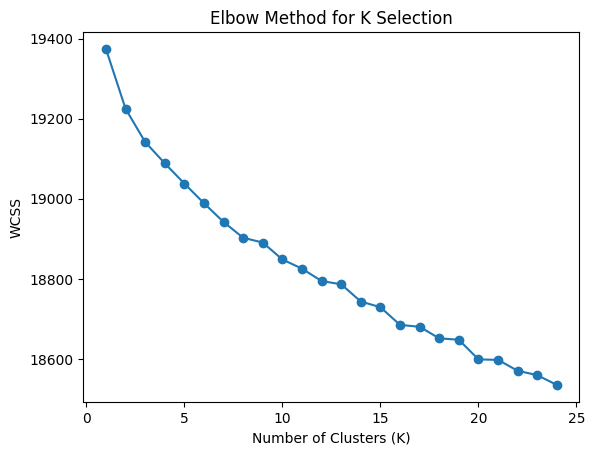
While the drop-off is not as steep as we would like to see, it seems that somewhere between 8 and 10 clusters is a good place to start. There is another technique called the Silhouette Coefficient that can be used to find the best K, so let's quickly look at that. The Silhouette Coefficient is a measure of how well samples are clustered. The Silhouette Coefficient is calculated for each sample, and the best value is the one with the highest silhouette coefficient:

from sklearn.decomposition import TruncatedSVD
from sklearn.cluster import KMeans
from sklearn.metrics import silhouette_score
import matplotlib.pyplot as plt

# reduce to ~100 dims for clustering/metrics
truncation = 100

n_comp = min(truncation, X.shape[1]-1)
X_svd = TruncatedSVD(n_components=n_comp, random_state=42).fit_transform(X)

ks = list(range(2, 25))
sil_scores = []
for k in ks:
    km = KMeans(n_clusters=k, random_state=42, n_init=10, max_iter=500)
    labels = km.fit_predict(X_svd)
    sil = silhouette_score(X_svd, labels)
    sil_scores.append(sil)

plt.plot(ks, sil_scores, marker='o')
plt.xlabel("K")
plt.ylabel("Silhouette score")
plt.title(f"Silhouette vs K (truncated at {truncation})")
plt.grid(True)
plt.show()

The code is very similar to our elbow graph code, except that for our silhouette graph we truncate the data to 100 components to denoise, speed up, and make distance computations more stable on high‑dim sparse TF‑IDF data. TruncatedSVD (LSA) projects TF‑IDF into a dense lower‑dim space that preserves the main semantic directions while removing noise and ultra‑sparse dimensions. While we could do the same for our elbow graph, it doesn't affect the results much (although it does speed up the computation).

After reducing the data to 100 dimensions, we then run the k-means algorithm, generate the silhouette score for each calculation, and plot them. But what is a silhouette score? It is a measure of how good the samples are clustered on a range from -1 → 1.

• ~+1 = well-matched to its own cluster, far from other clusters.
• 0 = on or near the boundary between clusters.
• ~–1 = possibly assigned to the wrong cluster.

The overall score is just the average silhouette value across all points. The silhouette score asks, for every point: “Am I closer to my own cluster than to the next nearest cluster?” Then it averages that across all points. If the answer is strongly “yes,” you get a high score. If clusters overlap, the score is low.

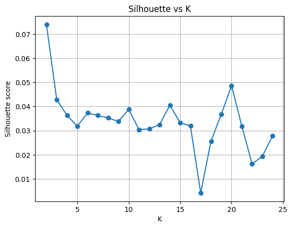
What you hope to see in a Silhouette graph is an obvious place in the graph where K is optimal. We can safely ignore values < 4, as they rarely produce good clusters; and our elbow chart (above) shows continuous improvement beyond K=2. The best our graph shows for truncation of 100 is a value of 20. However, if you experiment a bit with how much you truncate the date, you can see that different truncations (25, 50, 100, 150, 200) will give you different results. However, 20 does appear to be consistently one of the best K values.

Clustering the data (Step 2 — Fitting the model and saving artifacts)

Now that we have determined the best K value, we can use KMeans to cluster our data. We will use the same code as before, but we will use the best K value we found in the previous step, and we will also get the labels.

k = 20  # From the silhouette method and the elbow method k at 20 is the sweet spot.
kmeans = KMeans(n_clusters=k, random_state=42, n_init=10, max_iter=500)
labels = kmeans.fit_predict(X) 

print(f"Clustered into {k} groups.")

Now, through the magic of Jupyter notebooks, let's verify that we are getting some good results. In the following cell, we will get a random recipe from our list of titles and then find the top 5 recipes that are most similar to it. We will use the cosine similarity function to measure the similarity between the query and each of the top 5 recipes.

import random
import numpy as np
from sklearn.metrics.pairwise import cosine_similarity

top_n = 5

# Pick a random recipe to query.
rnd = random.Random()
idx = rnd.randrange(len(titles))
query_title = titles[idx]

# Find the top N similar recipes.
sims = cosine_similarity(X[idx], X).flatten()  # works with sparse X

# exclude the recipe we are querying from the top N results
sims[idx] = -1.0  

# Get the top N recipes by similarity, no need for effeciency here.
top_idx = np.argsort(sims)[::-1][:top_n]

# Output the results.
print(f"Query (index {idx}): {query_title}\nTop {top_n} similar recipes:")
for rank, i in enumerate(top_idx, start=1):
    fname = filenames[i] if 'filenames' in globals() else None
    print(f"{rank}. [{i}] {titles[i]} (score={sims[i]:.4f})" + (f" — file: {fname}" if fname else ""))

If we run this cell, we should see something like:

Query (index 17843): Instant Pot® Ribs
Top 5 similar recipes:
1. [16008] Baby Back Pork Ribs (score=0.4227) — file: recipe_16293.json
2. [15406] Instant Pot Ribs with White Barbecue Sauce (score=0.3035) — file: recipe_15691.json
3. [6410] Smoky Baby Back Ribs in the Crock-Pot (score=0.2995) — file: recipe_06437.json
4. [7473] Beef Bone Broth Recipe (score=0.2907) — file: recipe_07527.json
5. [7767] Crock Pot Baby Back Ribs (score=0.2632) — file: recipe_07825.json

This looks pretty good. We can see that the top 5 recipes are similar to the query recipe. We are using the cosine_similarity function in scikit-learn to measure the similarity the ingredients in the randomly picked recipe and recipes from our "database". Although we haven't seen it before, the cosine similarity is a measure of the similarity between two vectors, is a frequently used algorithm in machine learning. It is used in text analysis, for semantic search and RAG, face recognition, image deduplication, as well as the clustering example we are using here. The cosine similarity is defined as:

Cosine similarity (two equivalent forms)

$cosine(x,y) = \frac{x^\top y}{\lVert x \rVert \, \lVert y \rVert} = \frac{\sum_{i}^d x_i y_i}{\sqrt{\sum_{i}^d x_i^2}\;\sqrt{\sum_{i}^d y_i^2}}$

If vectors are L2-normalized

$cosine(\hat x,\hat y)=\hat x \cdot \hat y$

Cosine distance

$d_{\cos}(x,y)=1-cosine(x,y).$

If the actual formulae don't give you an intuition into what is going on, you can just think that the closer the result is to 1, the more similar the recipes are. As we will see in the FastAPI service in the next post, since TF-IDF vectors are L2-normalized, we can use the faster dot product shortcut rather than cosine similarity. However, for clarity and simplicity, we will use cosine similarity here since that is what we are actually calculating.

Now that we know that our we can save all the artifacts we have into our models' directory. We will save the k-means, the titles, the filenames, and the cluster assignments.

# Save artifacts
with open(project_root / "models/kmeans_model.pkl", "wb") as f:
    pickle.dump(kmeans, f)

with open(project_root / "models/recipe_titles.pkl", "wb") as f:
    pickle.dump(titles, f)

with open(project_root / "models/recipe_filenames.pkl", "wb") as f:   # <-- new
    pickle.dump(filenames, f)

# save the X matrix (can be large) so we don't need to recompute it
dump(X, project_root / "models/tfidf_matrix.joblib")   

Conclusion

Here’s where we landed: we cleaned ingredient text, turned each recipe into a TF‑IDF vector, used a little SVD to tame sparsity, picked a reasonable K with the elbow/silhouette duo, trained K‑Means, and used cosine similarity to pull “looks‑like this” recipes. This combo works nicely because cosine cares about proportions, not raw counts—perfect for ingredient lists with lots of small overlaps.

Along the way, we sanity‑checked clusters by looking at top terms and representative recipes, glanced at silhouette scores to confirm separation, and kept our artifacts (vectorizer, model, matrix) versioned together so runs stayed consistent. When clusters looked noisy, small tweaks (min_df/max_df or SVD size) helped clean things up. We also noted alternatives like spherical K‑Means or agglomerative clustering with cosine for future experiments.

In the next post we will look into creating a FastAPI endpoint that loads everything at startup and returns top‑K neighbors for any recipe title—complete with similarity scores and source filenames.